
A few weeks ago, Maxwell presented its data-driven financial materiality methodology to an industry workshop of reporters, assurers, investors and data platforms. On the day, the feedback was positive and the consensus was to move from proof-of-concept pilots to real world Beta projects.
As we roll out the Beta projects, we wanted to collect and share honest feedback from users.
This article sets out the general feedback that a methodology guide would be helpful. Other articles focus on the approach and on the reporter experience.
We welcome all feedback as we build out the product, please do let us know….. good and bad both welcome!
Why this matters if you work in sustainability reporting
The three-body approach answers the question: how much of a company's share price is driven by sustainability topics?
For anyone who works on materiality assessments, double materiality, assurance of sustainability disclosures or sustainable investing, the methodology solves for financial materiality. It offers a market-based view of which SASB topics investors are reacting to, which can be set alongside a company's own materiality assessment.
The approach is mathematical rather than driven by questionnaires so a typical report contains statistical vocabulary: betas, t-statistics, p-values, Ledoit-Wolf shrinkage, sandwich estimators, Sparsemax, Rank IC, NRMSE. This article explains each one in plain language, using numbers taken from four real reports (Admiral, BP, Microsoft and Next). No maths background is assumed. The purpose of this article is to explain what each figure means, so a lay reader knows which questions to ask before relying on the analysis for their use case.
2. The core idea: three bodies influencing one share price
The name borrows from Physics, where the "three-body problem" describes how three objects influence each other through gravity. Here, the the three bodies are:
• Sun — the market. The national benchmark index: the FTSE 100 for UK companies, the S&P 500 for US companies, and an equivalent for European ones. When the whole market rises or falls, most shares go with it.
• Moon — the sector. A custom index of the company's peers, for example "UK motor & home insurance" for Admiral or "Oil & Gas" for BP. Sector news (an oil price shock, a change in insurance regulation) moves all peers together.
• Earth — the company itself. Whatever is left after the market and sector have been accounted for. The model then allocates this company-specific part across SASB sustainability topics, using weekly sentiment scores for each topic.
One point is worth fixing in mind from the start, because it affects almost everything else: Sun and Moon are measured directly, while Earth is the remainder. That is why page 2 shows "N/A" for Earth's beta, t-stat and p-value. Earth is labelled "ESG", but strictly it is everything the market and sector do not explain, which the model then distributes across SASB topics.
3. The raw ingredients
The three-body analysis is built from the same four inputs, over a selected time window (typically 1 year, 3 years, 5 years as required).
1. Weekly log returns for the company. A "return" is the percentage change in price from one week to the next. A "log" return is a slightly different way of measuring that change which has one useful property: gains and losses of the same size cancel out exactly.
Example: a share goes from 100p to 110p, then back to 100p. Ordinary percentages say +10% then −9.1%, which looks like a net gain even though the price is back where it started. Log returns say +9.53% then −9.53%, which adds to zero. That makes weekly figures safe to add up and compare, which is why analysts prefer them.
2. Weekly log returns for the market index (Sun). The same calculation for the FTSE 100, S&P 500 or equivalent.
3. Weekly log returns for a sector peer index (Moon). The report query constructs a custom index from the company's peers, rebased to a starting value (BP's and Next's are rebased to 1,000).
4. Weekly SASB Polarity Balance Scores. For each SASB topic (GHG Emissions, Data Security, Labor Practices and so on), the company receives a weekly score. The score is calculated from the ratio of positive to negative relevant conversations in a given week. Microsoft's report, for example, describes weeks with more positive employee-sentiment coverage.
The SASB universe is 26 topics - 6 Environment, 10 Social and 10 Governance.
Data sourcing: inputs 1 and 2 are public market data. Inputs 3 and 4 are constructed by Maxwell Data from all the publicly-available conversation across traditional, trade and social media excluding what the company says about itself.
4. Reading the percentages
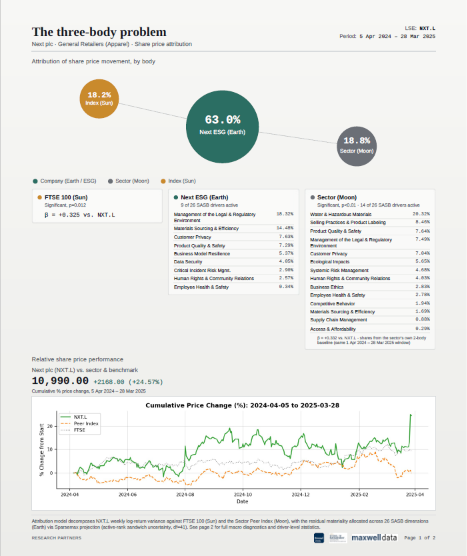
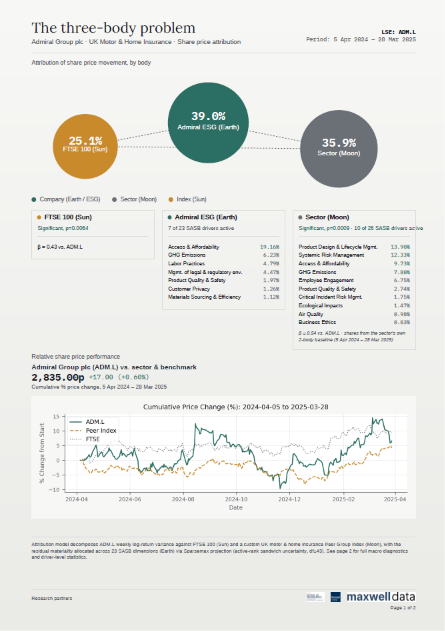
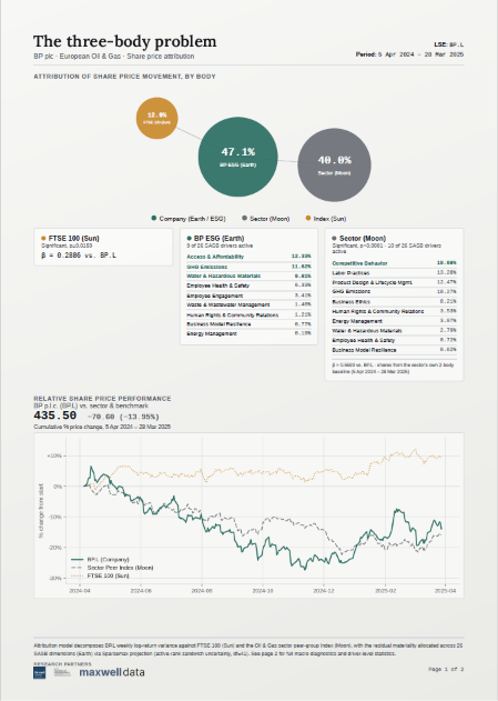
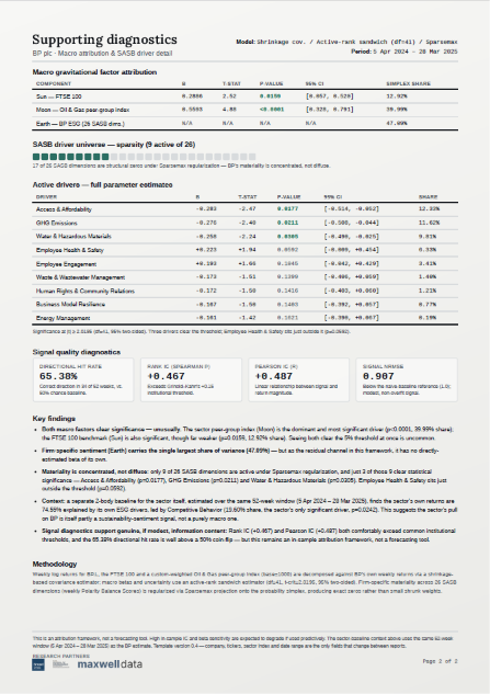
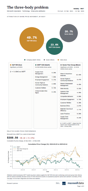
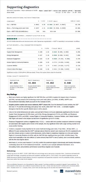
The headline percentages on page 1, repeated in the "Simplex share" column on page 2, divide the company's weekly share price movement between the three bodies. They are always zero or more and always add up to 100%. That is all "simplex" means: a set of shares of a whole, like slices of a pie.
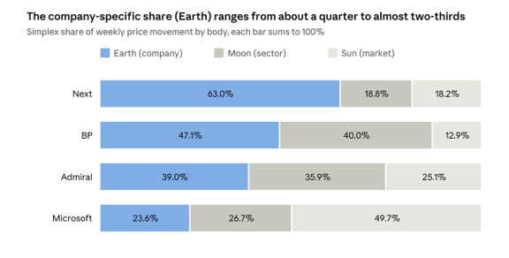
Page 2 'Simplex share' column of the Next, BP, Admiral and Microsoft reports · 52-week windows ending March 2025
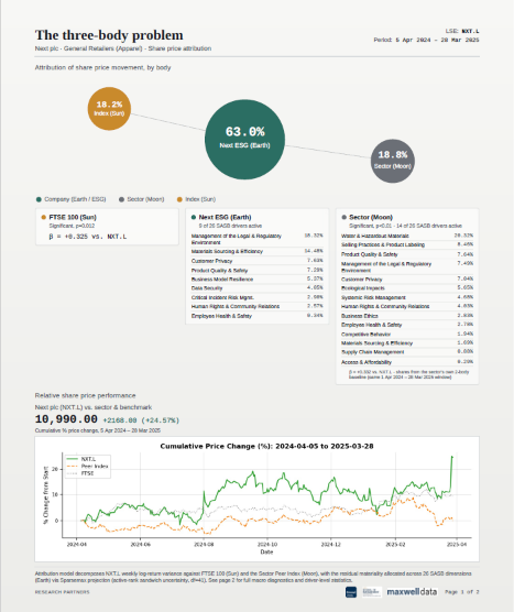
The split varies a great deal between companies. Microsoft's movement is dominated by the market: it largely moved with the S&P 500. Next sits at the other extreme, where nearly two-thirds of the movement is company-specific. BP and Admiral fall between, each with a strong sector pull.
How the SASB driver percentages relate to Earth
The driver percentages under Earth are slices of the Earth slice, not of the whole pie. Add them up and they come back to the Earth total. For Admiral, the seven active drivers (19.16% + 6.23% + 4.79% + 4.47% + 1.97% + 1.26% + 1.12%) sum to 39.01%, which is Admiral's Earth share. So "Access & Affordability 19.16%" means that topic accounts for about half of Admiral's company-specific movement, or about a fifth of its total movement.
The Moon driver list on page 1 is a different measure
The SASB list under "Sector (Moon)" on page 1 does not add up to the Moon share. It comes from a separate model of the sector index itself (explained in the walk-through below). Admiral's Moon drivers sum to 57.49%, the share of the sector's movement linked to the sector's sustainability topics. It is context about the peer group, not a further split of Admiral's 35.88%.
A percentage share is not the same as statistical confidence
A large share tells you how much of the movement a component is allocated. It does not tell you whether the evidence is strong. Admiral's GHG Emissions driver holds 6.23% of the movement but is not statistically significant. The next section explains how to tell the difference.
5. Four numbers in every row: β, t-stat, p-value and 95% CI
The tables on page 2 have the same five columns for every component and every SASB driver. Take Admiral's Sun row as a running example:

Beta (β): how strongly the share follows the factor
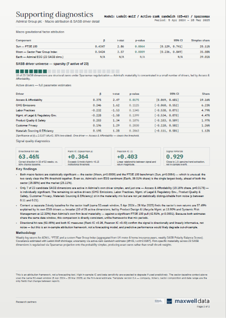
Beta measures sensitivity. Admiral's β of 0.43 against the FTSE 100 means that in a week when the FTSE 100 moves 1%, Admiral's share price tends to move about 0.43% in the same direction, once the sector has been accounted for.
• β = 1: moves one-for-one with the factor.
• β between 0 and 1: follows it, but more gently (Admiral, BP and Next against their indices).
• β negative: tends to move the opposite way.
For SASB drivers, the sign matters most. BP's GHG Emissions driver has β = −0.276. That means weeks with more positive GHG coverage tended to coincide with weaker BP share prices, and vice versa. To be clear: negative sign is a pattern in the data, not an explanation.
t-stat: how big the signal is compared with the noise
Every estimate comes with uncertainty, called its standard error. The t-stat is simply the beta divided by that uncertainty. Admiral's Sun t-stat of 2.86 means the estimated effect is 2.86 times larger than its own margin of error.
The rule of thumb in these reports: a t-stat beyond about ±2.02 counts as "significant". Each report prints the exact cut-off, for example |t| ≥ 2.0167 for Admiral. The value shifts slightly between reports because it depends on the degrees of freedom, explained in the next section.
p-value: how likely the result is to be a fluke
The p-value answers this question: if there were really no link at all, how often would we see a link at least this strong just by chance?
Admiral's Sun p-value is 0.0064, or 0.64%. Roughly 1 time in 156, pure chance would produce a pattern this strong. The reports use the conventional 5% (0.05) cut-off, so this counts as significant.
Compare BP's Employee Health & Safety driver, at p = 0.0592. That is a 5.9% chance of a fluke, just outside the cut-off. The report treats it as "not significant", though in practice it sits on the border.
A common misreading is worth avoiding. A p-value of 0.0064 does not mean there is a 99.36% chance the effect is real. It only says the data would be surprising if there were no effect.
95% confidence interval: the plausible range
The confidence interval (CI) gives the range of betas consistent with the data. Admiral's Sun interval is [0.129, 0.741]: the true sensitivity is plausibly anywhere from 0.13 to 0.74. That is a wide range, which is normal with only 52 weeks of data.
The quick test for significance: does the range include zero? If it does, "no effect" is still plausible.
• Admiral, Access & Affordability: [0.069, 0.681]. Zero is excluded, so it is significant (p = 0.0175).
• Admiral, GHG Emissions: [−0.060, 0.552]. Zero is included, so it is not significant (p = 0.1125).
The four numbers are tied together: β ± (cut-off × standard error) gives the interval. For Admiral's Sun row, 0.4347 ± (2.0167 × 0.152) gives 0.128 to 0.741, which matches the printed interval. That makes it a simple arithmetic check on any row.
6. The engine room: the model line on page 2
Each page 2 opens with a line such as Model: Ledoit-Wolf / Active-rank sandwich (df=43) / Sparsemax. These are three techniques, each solving a specific problem caused by having lots of candidate drivers and only one year of data.
The underlying problem: too many questions, too little data
The model has 52 weekly observations. It is trying to estimate effects for the market, the sector and up to 26 SASB topics. That is a bit like judging 28 restaurants from 52 meals: some estimates will look impressive purely by luck. All three techniques are ways of being more cautious with limited evidence.
Ledoit-Wolf shrinkage: tempering extreme estimates
The model first needs to know how all the inputs move together; statisticians call this the covariance. With few observations, raw covariance estimates are jumpy and exaggerate relationships.
Ledoit-Wolf shrinkage blends the raw estimate with a simpler, steadier "default" estimate. The method itself decides how much to blend, based on how noisy the data is.
Example: a new restaurant has three reviews, all five-star. A sensible diner does not conclude it is the best in town; they pull the rating partway toward the city average until more reviews arrive. Shrinkage does the same for the relationships between returns and sentiment scores.
Sandwich estimator: honest error bars
The standard formula for a standard error assumes every week is equally "noisy". Markets do not behave like that: some weeks are calm, others are turbulent. A sandwich estimator (named after the shape of its formula, with two identical "bread" terms around a "filling") produces error bars that remain reliable when volatility varies from week to week. In practice it tends to make the reported uncertainty more honest, usually wider.
Degrees of freedom (df): how much evidence is left over
Every item the model estimates "uses up" some of the data. Degrees of freedom are what remain to judge the results. In these reports the arithmetic is simple, and it reconciles exactly for every report we checked:
df = 52 weeks − 2 macro factors − number of active SASB drivers
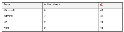
This is what "active-rank" means: only the drivers that survive into the model are counted. Fewer degrees of freedom means a slightly higher significance cut-off (2.0154 at df = 44, rising to 2.0195 at df = 41).
Sparsemax: forcing a clear materiality ranking
This is the technique that matters most for sustainability readers, because it produces the SASB driver list.
The model has to turn raw scores for each SASB topic into shares that are all zero or positive and add up to the Earth total. The common way of doing that, called softmax, gives every topic at least a small share. Sparsemax does the same job but sets weak topics to exactly zero.
A three-topic example with raw scores of 2.0, 1.2 and 0.1:
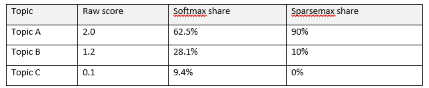
Softmax spreads materiality thinly across everything. Sparsemax produces a short list and drops the rest. The reports call those dropped topics "structural zeros". For BP, 17 of 26 topics are structural zeros and 9 are active.
Two cautions follow from this:
• A structural zero is not proof a topic is immaterial. It means the topic's sentiment did not track the share price closely enough, in this window, to earn a share.
• Active does not mean significant. Sparsemax decides which topics get a share; the t-stat and p-value decide whether the evidence is strong. Of BP's 9 active drivers, only 3 are significant. Of Next's 9, only 2 are.
7.Signal quality diagnostics: does the model fit the year it describes?
The four boxes near the bottom of page 2 ask one question in four ways: when the model's combined signal pointed up or down in a given week, did the share price agree?
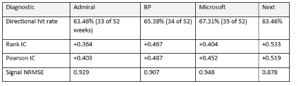
Directional hit rate: up or down, right or wrong
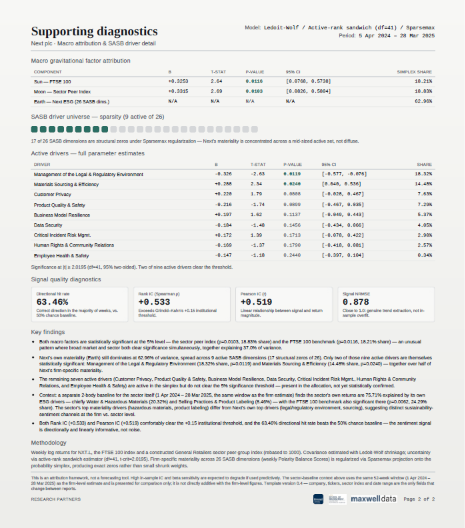
The simplest test. Each week, did the signal and the share price move in the same direction? Admiral's signal got the direction right in 33 of 52 weeks, or 63.46%. A coin toss would average 26 of 52 (50%), so the model does better than chance, though by around seven weeks a year, not by a landslide.
Rank IC (Spearman ρ): does the ordering match?
IC stands for "information coefficient". The Rank IC lines up the 52 weeks from the signal's strongest to its weakest, does the same for actual returns, and checks how similar the two orderings are. It runs from −1 (exactly opposite order) through 0 (no relationship) to +1 (identical order).
Example: if the signal ranked a week as its 5th-most-positive and the share had its 7th-best week, that is close agreement. If the share had its 48th-best week, that is poor agreement. Next's Rank IC of +0.533 means the orderings agree well; Admiral's +0.364 means moderately.
Pearson IC (r): does the size match too?
The Pearson IC is the ordinary correlation. It checks not just the order but whether bigger signals line up with bigger moves. It is on the same −1 to +1 scale.
A useful translation for non-specialists: squaring the correlation gives the share of week-to-week variation the signal "lines up with". Admiral's 0.403 squared is about 0.16, or roughly 16%. That is real, but it also shows most weekly movement remains unexplained.
Signal NRMSE: how big are the misses?
NRMSE (normalised root mean squared error) measures the typical size of the signal's errors, scaled so that 1.0 equals a simple "naive" benchmark. Below 1.0 means smaller errors than the benchmark.
Admiral's 0.929 means its errors are about 7% smaller than the naive benchmark. Next's 0.878 is about 12% smaller. The reports present values close to 1.0 as reassurance that the model is not over-fitted, which is fair. The other side of the same coin is that the improvement in magnitude is modest, even though direction and ordering are good.
What the "+0.15 institutional threshold" does and does not mean
Grinold and Kahn's widely quoted rules of thumb apply to genuine forecasts, tested on data the model has not seen. These reports measure fit within the same year used to build the model, which is described as in-sample. In-sample ICs are almost always higher. The reports themselves state that performance would likely degrade if used predictively, and this caveat matters more than the comparison.
8. How the insights are derived: a walk-through of Next plc
The "Key findings" in each report follow the same six-step logic. Here it is applied to Next, whose share price rose 24.57% over the window.
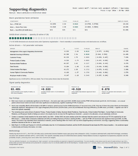
Step 1: Are the market and sector links real? Check the p-values for Sun and Moon. Next's are 0.0116 and 0.0103, both below 0.05, so both links are significant. The reports often remark that this is unusual; together the two explain 37.0% (18.21% + 18.83%).
Step 2: How big is the company-specific part? Earth is 62.96%, the remainder. So most of Next's weekly movement did not follow the FTSE 100 or its retail peers. This is the headline: Next's share price behaved largely on its own terms.
Step 3: Which SASB topics carry that company-specific part? Sparsemax kept 9 of 26 topics. The largest shares are Management of the Legal & Regulatory Environment (18.32%) and Materials Sourcing & Efficiency (14.48%). Together they account for just over half of Earth.
Step 4: Which of those are statistically supported? Only those two clear the significance cut-off (p = 0.0119 and 0.0240). The other seven are present in the allocation but could be noise.
Step 5: Which way do they point? Materials Sourcing has a positive beta (+0.288): better sourcing coverage coincided with better share price weeks. Legal & Regulatory has a negative beta (−0.326): weeks with more positive coverage on this topic coincided with weaker share price weeks. A negative sign often surprises readers. It may reflect timing (markets reacting before coverage turns), or coverage that reads as positive but signals cost. The model cannot say which.
Step 6: Compare with the sector. Each report also runs a separate, simpler "2-body" model on the sector index itself (market plus the sector's own SASB topics, no Moon). For Next's sector, ESG sentiment explains 75.71%, led by Water & Hazardous Materials (20.32%). Next's own top topics differ from the sector's, so the report concludes that the firm and its sector respond to different sustainability themes.
What this tells a materiality practitioner: market sentiment around Next appears to respond most to legal and regulatory matters and to materials sourcing. If the company's own materiality assessment ranks these topics low, that is a prompt for a conversation, not a conclusion. It is a single year of in-sample data, and the model identifies patterns, not causes.
9.Limits, and the questions an assurance practitioner should ask
The analysis describes the past rather than predicts the future. For anyone placing reliance on them, a few further points deserve attention.
1. Earth is a remainder, not a direct measurement of ESG. Earth captures everything the market and sector do not, including earnings surprises, management changes and takeover speculation. The model then distributes that remainder across SASB topics. A large Earth share therefore means "strongly company-specific", which is not automatically the same as "strongly ESG-driven". This matters for any analysis that compares Earth with Moon, such as ranking companies as higher risk when Earth exceeds Moon: that comparison measures how idiosyncratic a share is relative to its sector, and labelling it ESG risk relies on the SASB allocation being meaningful.
2. Many tests, one year: expect some false positives. With 26 topics each tested at the 5% level, about one topic per report could look significant purely by chance. A single significant driver at p = 0.03 deserves less weight than its p-value suggests. Drivers at p < 0.01, or repeating across years, deserve more.
3. The Moon driver list on page 1 is easy to misread. Its percentages come from the sector's own 2-body model. They add up to the sector's ESG share (57.49% for Admiral's sector), not to the company's Moon share (35.88%). They describe the sector, not the company.
10.Glossary
-
Weekly % price change, measured so gains and losses of equal size cancel out
Example: 100p → 110p → 100p nets to zero
-
Market index / sector peer index / company-specific remainder
Example: FTSE 100 / Oil & Gas peers / BP
-
A set of shares, all zero or more, that add up to 100%
Example: Admiral: 25.11% + 35.88% + 39.01%
-
How much the share moves when the factor moves 1%
Example: Admiral vs FTSE 100: 0.43
-
Size of the effect divided by its margin of error; beyond about ±2.02 is significant
Example: Admiral Sun: 2.86
-
Chance of seeing a link this strong if none existed; below 0.05 is significant
Example: Admiral Sun: 0.0064
-
Plausible range for β; significant if it excludes zero
Example: Admiral Sun: 0.129 to 0.741
-
Data left over after estimating; here 52 − 2 − active drivers
Example: Admiral: 43
-
Pulls jumpy estimates toward a steadier default
Example: Like averaging a new restaurant's reviews with the city average
-
Error bars that stay reliable when some weeks are more volatile
Example: Used for every p-value and CI
-
Turns topic scores into shares, setting weak topics to exactly zero
Example: BP: 9 active, 17 structural zeros
-
A SASB topic given no share in this window
Example: 20 of 26 topics for Microsoft
-
Separate model of the sector index: market + sector SASB topics
Example: Next's sector: 75.71% ESG
-
% of weeks where signal and price moved the same way; 50% = chance
Example: Microsoft: 35 of 52 weeks
-
Agreement between signal and returns in order / in size, from −1 to +1
Example: Next: +0.533 / +0.519
-
Typical error size; 1.0 = naive benchmark, lower is better
Example: BP: 0.907